Computational Stylistics Group | Using the function stylo() in batch mode

Introduction

The stylometric package stylo is known mostly for its main function, namely stylo(), which is a do-it-all-at-once piece of software to be run in interactive mode. Advanced users sooner or later discover other functions such as classify(), oppose() etc., let alone lower-level functions to perform text-preprocessing. Conveniently, all these functions can serve as building blocks to design your own experiment, which might be run on a server in batch mode (by running a script, rather than via GUI). Some of the above functionalities are covered in previous posts.

A natural question can be asked whether the main function stylo() exhibits similar properties: is it possible to invoke it from inside a script, and run on a server in batch mode? A short answer is yes, it is possible, for two different reasons. Firstly, all the R functions can be evaluated in such a way that whatever they return is piped into a variable, e.g.:

my_new_variable = stylo()

From now on, the object my_new_variable will store the output of the function stylo() (no plots, though). Secondly, the function stylo() can silence its GUI interface by using a dedicated argument. Consequently, all the other parameters of the model can be passed as command-line arguments, e.g.:

another_variable = stylo(gui = FALSE, mfw.min = 200, mfw.max = 200)

The above call will read input texts from files, and then perform a default analysis (hierarchical clustering, Classic Delta similarity measure) with 200 most frequent words as stylometric features. By adding additional arguments, one is able to set the linkage method, visualization flavor (or choose to silence the visualizations); one can even use the already existing table of word frequencies without loading the input texts from the files.

To test the applicability of the function stylo() in batch mode, let’s attack a relatively simple problem which is however very rarely reported in literature. Namely, we will address the question to which extent stylometric distance between two different texts is stable. Certainly, several studies have shown that the final results depend on the choice of the features – the picture for 100 most frequent words is different than that for 1,000 most frequent words – but there is still very little awareness of what it really means, statistically.

In the following sections we will gradually build a script to perform a real-life experiment testing the similarities between different texts in a corpus. We will start with a simple scenario involving just two texts: we will examine the variability of the distance between them given different input features.

What is a distance between two given texts, really?

The idea is simple. From a pool of available features (here: most frequent words), we randomly select, say, 100 of them, and compare the two input texts using the function stylo(). Then we repeat the procedure and record the resulting distance. Then we observe the statistical properties of the obtained distances.

To randomly select n elements from the pool of features, we can use the generic function sample(). E.g. if we want to draw 10 elements from the range 1:100, we type:

sample(1:100, 10)

##  [1]  71   5  27  94  44  92  85  74   9 100

Now, the goal is to put all the pieces together. We aim to perform 100 iterations, and in each iteration we aim to estimate the distance between two texts from the lee dataset. As an example, we’ll use the 1^st and the 2^nd text, e.g. In Cold Blood by Truman Capote, and Breakfast at Tiffany’s by the same author. We run the loop 100 times, and in each turn we run the function stylo() with frequencies of randomly selected 100 features. Once a loop is complete, we collect the results.

The dataset lee is provided by the package stylo. It is a matrix with word frequencies of 3,000 MFWs for 28 American novels. Type help(lee) to see what’s inside.

library(stylo)
data(lee)
final.results = c()

for(iteration in 1:100) {

    # randomly pick 100 numbers from the range 1:3000
    pick.features = sample(1:3000, 100, replace = FALSE)
    # select the features matching the 100 random numbers
    dataset = lee[ , pick.features]
    # perform the unsupervised classification, using Classic Delta
    results = stylo(frequencies = dataset, gui = FALSE, display.on.screen = FALSE)
    # pick the distance stored in the 1st row and 2nd column,
    # e.g. the one between two different texts by Capote
    final.distance = results$distance.table[1,2]
    # add the new results to the already existing vector
    final.results = c(final.results, final.distance)

}

The collected 100 distances are stored in the variable final.results. Basic statistics include the mean of all the distances and the standard deviation:

mean(final.results)

## [1] 0.8665739

sd(final.results)

## [1] 0.09405702

The arithmetic mean is often considered a good proxy for the actual distance between two texts. However, the realization of how big is a dispersion between the shortest and the longest distance between the same pair of texts might be really disappointing:

min(final.results)

## [1] 0.6417331

max(final.results)

## [1] 1.123667

Quite a spread, huh? A better insight into the results will be provided by estimating the distribution of the computed 100 distances. A simple density plot will support the interpretation:

distances = density(final.results)
plot(distances, main = "Two novels by Capote")

Distances between <i>In Cold Blood</i> by Truman Capote, and <i>Breakfast at Tiffany’s</i> by the same author. Classic Delta used as a distance measure.

Take the results obtained so far, as a caveat. The distance between a given pair of texts might vary quite a lot, depending on the choice of input features. Also, it will depend on the number of features tested at a time. Try to edit the above code, so that in each iteration 1,000 random features are drawn instead of 100 features. (Edit the line that invokes the function sample()). How will the observed distribution change?

The distribution of distances in a corpus

Now, what if we generalize the above code to cover all the texts in the corpus? The idea is to examine all pairwise distances between available texts, in order to see how wide the final distribution might be. The code discussed in the previous section needs but a minor tweak to achieve the goal:

library(stylo)
data(lee)
final.results = c()

for(iteration in 1:100) {

    pick.features = sample(1:3000, 100)
    dataset = lee[ , pick.features]
    results = stylo(frequencies = dataset, gui = FALSE, display.on.screen = FALSE)
    final.distance = as.vector(results$distance.table)
    final.results = c(final.results, final.distance)

}

# since the values contain self-similarity tests as well, 
# here's a dirty trick to get rid of 0 values from the results:
final.results = final.results[final.results > 0]

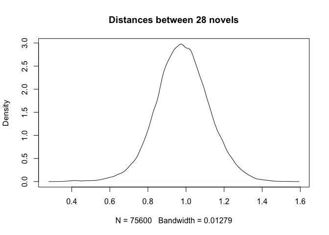
Again, we plot the distribution:

distances = density(final.results)
plot(distances, main = "Distances between 28 novels")

Distances between all possible pairs of texts in the corpus of 28 English novels.

Quite striking is the observation that we deal here with a normal (or Gaussian) distribution, while in fact the pairwise comparisons involved (i) pairs of texts by the same author and (ii) pairs of texts by different authors. We should expect the first group to be narrower and the second group to be wider, and above all, we should expect to see a bi-modal distribution (i.e. with two humps) rather than a Gaussian one. The next session will address the issue.

Putting it all together

The final version of the script will resemble a typical authorship verification procedure. In short, here we will split the distances into the ones generated by texts of the same authorship (ingroup distribution), and texts of different authorship (outgroup distribution). For the sake of convenience, the preamble contains the settings to be adjusted in a real-life series of tests. Here’s the code:

library(stylo)
data(lee)

####### adjust the parameters #############

# pick a distance: "delta", "wurzburg", ...
preferred.distance = "wurzburg" 

# choose a number of randomly picked features
random.features = 100

###########################################


final.results.same = c()
final.results.different = c()

for(iteration in 1:100) {

    pick.features = sample(1:3000, random.features)
    dataset = lee[ , pick.features]
    results = stylo(frequencies = dataset, gui = FALSE, display.on.screen = FALSE, mfw.min = 3000, mfw.max = 3000, distance.measure = preferred.distance)

    final.distance = results$distance.table

    classes = gsub("_.*", "", rownames(final.distance))

    for(n in 1:length(classes) ) {

        same = classes[n] == classes
        different = classes[n] != classes
        same.distance = final.distance[n, same]
        different.distance = final.distance[n, different]

    }

    final.results.same = c(final.results.same, same.distance)
    final.results.same = final.results.same[final.results.same > 0]
    final.results.different = c(final.results.different, different.distance)

}

# estimating the density funcion
density.same = density(final.results.same)
density.different = density(final.results.different)

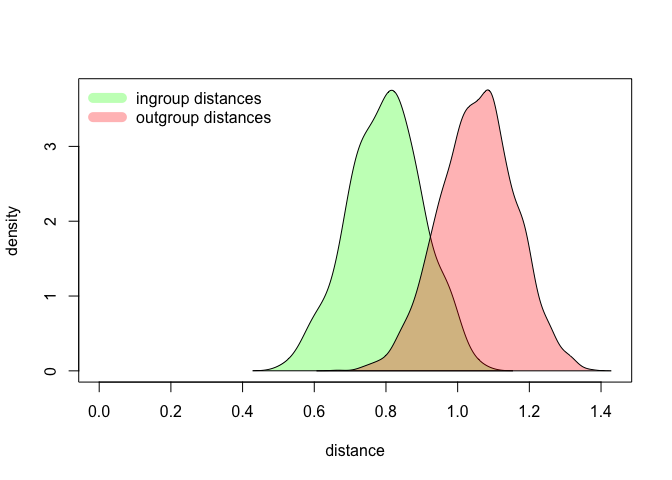
We have completed a very solid test. (Seriously, it’s a real, fully-fledged setup that can be used in an actual publication). It deserves a plot somewhat more sophisticated than the plots presented in the previous sections. I encourage you to analyze the following code yourself, nonetheless worth mentioning are: semi-transparent colors set in the first lines (fancy.green, fancy.red), determining the range of the plot (max.y.value, max.x.value), calling an empty scatterplot (plot(NULL)), adding colored areas representing the distributions (polygon()), and finally adding a legend to the plot (legend()). Here it is:

# plotting the outgroup and the ingroup distances
fancy.green = rgb(0, 1, 0, 0.3)
fancy.red = rgb(1, 0, 0, 0.3)
max.y.value = max(c(density.same$y, density.different$y))
max.x.value = max(c(density.same$x, density.different$x))
plot(NULL, ylim = c(0, max.y.value), xlim = c(0, max.x.value), ylab = "density", xlab = "distance")
polygon(density.same, col = fancy.green)
polygon(density.different, col = fancy.red)
legend("topleft", legend = c("ingroup distances", "outgroup distances"), lty = 1, lwd = 10, col = c(fancy.green, fancy.red), bty = "n")

Distances between ingroup and outgroup texts in the corpus.

Again, try to replicate the test with different settings, e.g. different distance measures, or different number of features. As you will see, some parameters make the two distributions more distinct, whereas other settings barely differentiate the subsets. Try to determine the optimal set of parameters, and do find a moment to think why some factors play a role in making the authorial signals distinct.