Performance measures in supervised classification
In this post, I provide a concise introduction to evaluation measures
for supervised machine-learning classification that are implemented in
the package stylo. In ver. >0.7.3 of the package, there exists the
function performance.measures() that is meant to be used in
combination with classification functions such as classify(),
perform.svm(), perform.delta(), or crossv().
Introduction
In supervised classification, assessing the quality of the model is of a paramount importance. To cut long story short, the following question has to be addressed when the classification results are concerned: how do I know whether my outcomes are good enough? How do I distinguish acceptable from unsatisfactory?
The basic idea behind model evaluation in machine learning is that before we apply our method to a sample (a text) to be actually classified, we perform a series of tests using a number of samples we already know where they should belong. However, we pretend we don’t know the expected answer, and we make the computer perform the classification. This allows us to asses to what extent the so-called ground truth matches the outcomes predicted by the computer. The higher the match between the actual and the predicted values, the more efficient the classification scenario under scrutiny. Put simply, such an evaluation procedure gives us a hint on how reliable the future results on new samples are likely to be.
A tl;dr working example
In this nutshell-style example, we’ll use the table with word
frequencies that is provided by the package stylo. First and foremost,
we need to activate the package, and then to activate the dataset lee
by typing:
library(stylo)
data(lee)
Next, we run a supervised classification with cross-validation. We will
use the leave-one-out scenario that is provided by the function
crossv(), and will leave the default settings. Unless other
classification method is specified, the function performs Classic Delta.
results = crossv(training.set = lee, cv.mode = "leaveoneout")
The classification task is completed but the fun part is yet to come. The following function gives you the report of the classifier’s behavior:
performance.measures(results)
## $precision
##    Capote  Faulkner   Glasgow HarperLee McCullers   OConnor    Styron     Welty
##      1.00      1.00      1.00      1.00      1.00      0.75      0.80      1.00
##
## $recall
##    Capote  Faulkner   Glasgow HarperLee McCullers   OConnor    Styron     Welty
## 0.8000000 1.0000000 1.0000000 1.0000000 0.6666667 1.0000000 1.0000000 1.0000000
##
## $f
##    Capote  Faulkner   Glasgow HarperLee McCullers   OConnor    Styron     Welty
## 0.8888889 1.0000000 1.0000000 1.0000000 0.8000000 0.8571429 0.8888889 1.0000000
##
## $accuracy
## [1] 0.9285714
##
## $avg.precision
## [1] 0.94375
##
## $avg.recall
## [1] 0.9333333
##
## $avg.f
## [1] 0.9293651
In a vast majority of real-life applications, however, the users choose
to load their texts directly from files, and then proceed with the
default tokenization procedure provided by the function classify(). In
such a case, follow your daily routine and add one additional step at
the end:
my_results = classify()
performance.measures(my_results)
What you get is the values of accuracy, recall, precision, and F1, which will be discussed below in detail.
Typical scenarios
In supervised machine-learning, the classification procedure is divided
into two steps. Firstly, a selection of texts belonging to known classes
is picked in order to train a model, and only then the remaining texts
are compared against the already-trained classes. A usual routine using
the package stylo starts with creating two subdirectories in the
filesystem:
- subdirectory
primary_setfor the training set files, - subdirectory
secondary_setfor the validation (test) set files.
The respective files should then be copied to the primary_set (here
goes the training material) and the secondary_set (the validation
material and the samples to be tested). Now, having specified the
working directory, type:
classify()
… and then specify your input parameters using graphical user interface
(GUI) that pops up when the function is launched. However, in order to
assess the overall behavior of the classification, it is recommended to
pipe the outcomes of the function classify() into a variable, so that
the results don’t simply evaporate, e.g.:
my_cool_results = classify()
Moreover, in machine-learning it is usually recommended to use cross-validation. This technique greatly increases the reliability of the final results, yet it comes at the cost of a substantially longer computation time (for more details see the post on using cross-validation). To classify the corpus using 10-fold stratified cross-validation, type:
my_cool_results = classify(cv.folds = 10)
If you use the above procedure in your projects and/or you know how to
use the function crossv() that requires some more care, then you can
skip the next paragraphs and go directly to the section Performance
measures. However, if you want to copy-paste
some snippets of code and get dummy results without preparing your own
corpus, the following examples are for you. For replicability reasons,
below we will be using an already existing dataset which is a part of
the package stylo. The code should be replicable on any machine.
First, we activate the package, and then the dataset, by typing:
library(stylo)
data(lee)
The dataset contains word frequencies for 3,000 most frequent words
(MFWs), extracted from 28 novels by 8 authors from the American South.
For the sake of simplicity, we will use the entire lee frequency table
with its 28 texts and 3,000 most frequent words, but feel free to
experiment with the size of the dataset, too.
In machine-learning terminology, each of the 28 texts belongs to one of the 8 classes. We need to take at least one text per class into the training set. To make the task more difficult for the classifier, we’ll take exactly one text per class. We can choose from the following novels:
rownames(lee)
##  [1] "Capote_Blood_1966"          "Capote_Breakfast_1958"
##  [3] "Capote_Crossing_1950"       "Capote_Harp_1951"
##  [5] "Capote_Voices_1948"         "Faulkner_Absalom_1936"
##  [7] "Faulkner_Dying_1930"        "Faulkner_Light_1832"
##  [9] "Faulkner_Moses_1942"        "Faulkner_Sound_1929"
## [11] "Glasgow_Phases_1898"        "Glasgow_Vein_1935"
## [13] "Glasgow_Virginia_1913"      "HarperLee_Mockingbird_1960"
## [15] "HarperLee_Watchman_2015"    "McCullers_HeartIsaLo_1940"
## [17] "McCullers_Member_1946"      "McCullers_Reflection_1941"
## [19] "OConnor_Everything_1956"    "OConnor_Stories_1960"
## [21] "OConnor_WiseBlood_1949"     "Styron_Choice_1979"
## [23] "Styron_Darkness_1951"       "Styron_House_1960"
## [25] "Styron_Turner_1967"         "Welty_Delta_1945"
## [27] "Welty_Losing_1946"          "Welty_TheOptimis_1969"
As you must have noticed, the class IDs are hidden in the names of the
samples: any string of characters before the first underscore is
considered to be a discrete class ID, e.g. McCullers or Faulkner.
Our selection of the training samples might include the following items
c(1, 6, 11, 14, 16, 19, 22, 26) (or whatever is your choice); these
texts will go to the training set:
training_set = lee[c(1, 6, 11, 14, 16, 19, 22, 26), 1:100]
Mind that we indicated 8 rows from the original dataset (out of 28). As
to the columns, the new subset training_set will contain the first 100
out of 3,000, since we selected the columns 1:100. Obviously, this
means that the analysis will be restricted to 100 most frequent words.
The size of the resulting training set matrix will be then 8 texts *
100 words. If you don’t believe, you can check it yourself:
dim(training_set)
## [1] 8 100
When it comes to the test set, we’d like to select all the remaining texts (i.e. rows). The number of columns will need to be trimmed as well, in order to match the 100 columns of the training set. Mind the minus sign to indicate the rows not listed in the index:
test_set = lee[-c(1, 6, 11, 14, 16, 19, 22, 26), 1:100]
We’re ready to launch the classification. When loading the texts from
files, one would use the function classify() without any arguments (as
described above). In our case, we have to indicate the already existing
training set and the test set. Additionally, we can silence the
graphical user interface (GUI):
results = classify(gui = FALSE, training.frequencies = training_set, test.frequencies = test_set)
Apart from the normal behavior of the function classify(), which
concisely reports the classification results into the file
final_results.txt, the newly created R object results contains much
richer information about the outcomes of the procedure. Depending on the
classification method used, these variables might look different. In
order to see what’s actually there, type:
summary(results)
##
## Function call:
## classify(gui = FALSE, training.frequencies = training_set, test.frequencies = test_set)
##
## Available variables:
##
##            distance.table  final distances between each pair of samples
##                  expected  ground truth, or a vector of expected classes
##                  features  features (e.g. words, n-grams, ...) applied to data
##    features.actually.used  features (e.g. frequent words) actually analyzed
##     frequencies.both.sets  frequencies of words/features accross the corpus
##      frequencies.test.set  frequencies of words/features in the test set
##  frequencies.training.set  frequencies of words/features in the training set
##                 predicted  a vector of classes predicted by the classifier
##              success.rate  percentage of correctly guessed samples
##
## These variables can be accessed by typing e.g.:
##
##    results$distance.table
To get any of the listed variables, follow the standard R convention of
using $. E.g. try the following code yourself:
results$features
In a similar way, you can have an access to all the other variables that
are stored within our newly created object results. Importantly, the
object contains some relevant information to assess the model’s quality.
Performance measures
Let’s jump directly to the meet-and-potatoes. The package stylo ver.
>0.7.3 provides a convenience function that does for you all that is
needed:
performance.measures(results)
## $precision
##    Capote  Faulkner   Glasgow HarperLee McCullers   OConnor    Styron     Welty
## 0.8000000 1.0000000 0.0000000 0.3333333 0.5000000 1.0000000 0.6666667 1.0000000
##
## $recall
##    Capote  Faulkner   Glasgow HarperLee McCullers   OConnor    Styron     Welty
## 1.0000000 0.2500000 0.0000000 1.0000000 1.0000000 1.0000000 0.6666667 1.0000000
##
## $f
##    Capote  Faulkner   Glasgow HarperLee McCullers   OConnor    Styron     Welty
## 0.8888889 0.4000000 0.0000000 0.5000000 0.6666667 1.0000000 0.6666667 1.0000000
##
## $accuracy
## [1] 0.7
##
## $avg.precision
## [1] 0.6625
##
## $avg.recall
## [1] 0.7395833
##
## $avg.f
## [1] 0.6402778
A good share of stylometric papers report just one measure, namely accuracy. Simply put, this is the number of correctly recognized samples divided by the total number of samples. Since in our example we have 20 texts in the test set, and the reported accuracy is 0.7, it means that 14 texts must have been correctly recognized. In the real world of machine-learning, however, this might be insufficient. Being conceptually very simple and compact, accuracy is considered to overestimate the actual classification performance. For this reason, a routinely applied toolbox of measures not only includes accuracy, but also recall, precision, and particularly the F1 score.
Recall tells us how many correct samples were harvested by the classifier (therefore you can think of this measure as of a sensitivity indicator), while precision reports how many texts assigned to a given class, were correct hits. Low recall scores betray a blind classifier, whereas low precision indicates that a classifier was too greedy. The F1 score combines the information from both recall and precision, and for that reason it is widely used to report the overall performance of classification.
The reason why these somewhat less intuitive measures are often
neglected in stylometric studies, is that they are not designed for
assessing multi-class scenarios. Since in our experiment 8 authorial
classes were involved, the recall, precision, and the F1 were reported
independently for each class. Not very convenient, uh? Look at the
numbers at the bottom: the avg.precision, avg.recall and avg.f are
the macro-averaged versions of precision, recall and the F1 score,
respectively. I encourage you to consult the help page for further
details, especially when the F1 or, say, F2 score is concerned:
help(performance.measures)
The information provided so far allows you to conduct successful experiments. Don’t stop reading, however, if you want to learn how the intermediate stages between the classification itself and the final performance scores are computed. First and foremost, the classifier goes over the test set and for each sample, it tries to guess where the sample should belong. Consequently, we obtain two rows of values (usually IDs), one is the sequence of classes that we know are true, and the second that the classifier thinks is true. The first is referred to as the expected values, while the second – the predicted values. Here’s how they look like:
results$predicted
##  [1] "Capote"    "Capote"    "Capote"    "Capote"    "HarperLee" "McCullers"
##  [7] "Faulkner"  "HarperLee" "Capote"    "Styron"    "HarperLee" "McCullers"
## [13] "McCullers" "OConnor"   "OConnor"   "McCullers" "Styron"    "Styron"
## [19] "Welty"     "Welty"
## attr(,"description")
## [1] "a vector of classes predicted by the classifier"
results$expected
##  [1] "Capote"    "Capote"    "Capote"    "Capote"    "Faulkner"  "Faulkner"
##  [7] "Faulkner"  "Faulkner"  "Glasgow"   "Glasgow"   "HarperLee" "McCullers"
## [13] "McCullers" "OConnor"   "OConnor"   "Styron"    "Styron"    "Styron"
## [19] "Welty"     "Welty"
## attr(,"description")
## [1] "ground truth, or a vector of expected classes"
As you can see, e.g. the ground truth for the 5th sample was Faulkner
but the classifier decided it to be HarperLee instead. (The question
why Lee was mistaken for Faulkner is worth a separate discussion, which
I’ll skip here). There are 6 mistakes overall. Not very impressive, to
be honest. Useful as it is, the overall performance does not say a word
about the particular texts’ behavior. A very convenient way to present
the expected and the predicted values is a confusion matrix, as in the
following example:
table(results$expected, results$predicted)
##
##             Capote Faulkner HarperLee McCullers OConnor Styron Welty
##   Capote         4        0         0         0       0      0     0
##   Faulkner       0        1         2         1       0      0     0
##   Glasgow        1        0         0         0       0      1     0
##   HarperLee      0        0         1         0       0      0     0
##   McCullers      0        0         0         2       0      0     0
##   OConnor        0        0         0         0       2      0     0
##   Styron         0        0         0         1       0      2     0
##   Welty          0        0         0         0       0      0     2
The numbers indicate the tallies of texts assigned to particular classes. The matrix is not symmetrical, so be careful not to confuse the rows and the columns. The rows contain the information about the expected (actual) classes, while the columns store the predictions of the classifier. In an ideal world, all the non-zero values should flock along the diagonal (thus indicating a perfect classification), but it is rarely the case. The recall and precision values give us a compact insight into the possible performance glitches. The way in which one computes recall and precision will not be discussed here: it’s a straightforward and standardized procedure (e.g. see the Wiki page for details).
As mentioned above, the machine-learning world is obsessed with the concept of reliability. How can we know that our training set is representative enough for the 8 authorial classes? We can’t. However, we can perform our test several times with randomly swapped texts from the training and the test set, and observe an average behavior of the corpus. Here’s our setup with 100-fold cross-validation switched on:
results2 = classify(gui = FALSE, training.frequencies = training_set,
                    test.frequencies = test_set, cv.folds = 100)

performance.measures(results2)
## $precision
##    Capote  Faulkner   Glasgow HarperLee McCullers   OConnor    Styron     Welty
## 0.7882600 1.0000000 0.8818898 0.6756757 0.6612022 0.6297468 0.7244582 0.7539062
##
## $recall
##    Capote  Faulkner   Glasgow HarperLee McCullers   OConnor    Styron     Welty
##     0.940     0.425     0.560     1.000     0.605     0.995     0.780     0.965
##
## $f
##    Capote  Faulkner   Glasgow HarperLee McCullers   OConnor    Styron     Welty
## 0.8574686 0.5964912 0.6850153 0.8064516 0.6318538 0.7713178 0.7512039 0.8464912
##
## $accuracy
## [1] 0.7525
##
## $avg.precision
## [1] 0.7643924
##
## $avg.recall
## [1] 0.78375
##
## $avg.f
## [1] 0.7432867
This time the diagnostic values are somewhat higher than in the previous example, and probably more likely to exhibit the actual behavior of the corpus. This is due to the fact that cross-validation examines many different compositions of the training set and the test, and consequently minimizes the effect of local idiosyncrasies. Diagnostic scores based on just one snapshot – as in the previous example – might lead to overly optimistic (or overly pessimistic) conclusions. Cross-validation is designed to mitigate the risk. Mind the high number of performed classifications:
table(results2$expected, results2$predicted)
##
##             Capote Faulkner Glasgow HarperLee McCullers OConnor Styron Welty
##   Capote       376        0       0         1         0       0     23     0
##   Faulkner      12      170       6        41        55      56     21    39
##   Glasgow       46        0     112         1         1       8     23     9
##   HarperLee      0        0       0       100         0       0      0     0
##   McCullers      2        0       2         0       121      49     19     7
##   OConnor        0        0       0         0         1     199      0     0
##   Styron        41        0       7         5         5       0    234     8
##   Welty          0        0       0         0         0       4      3   193
Certainly, the total number of actual texts has never changed, but
these 20 texts were scrutinized several times in 100 cross-validation
folds. Particular texts were randomly assigned either to the training
set, or to the test set, but on average each text was classified ca.
100 times. As an exercise, try to assess the total number of individual
tests performed (hint: apply the function sum() to the above confusion
matrix).
A working example
Let’s try something more ambitious. I mentioned in the previous section
that accuracy exhibits a tendency to overrate the actual performance,
therefore other measures should be reported too, preferably the F1
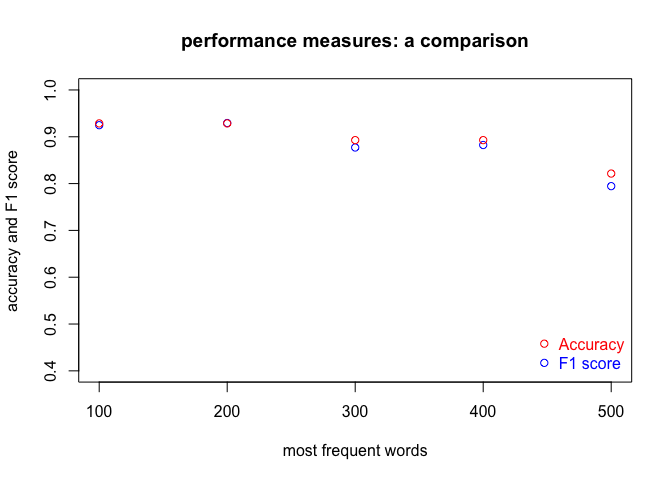
score. The following test will empirically examine the (hypothesized)
divergence between these two measures in a systematic way. Also, we will
introduce another variable to the equation, namely the number of most
frequent words to be tested. It has been shown in many studies that
longer vectors of MFWs usually increase the performance, but after a
certain point the performance gradually drops as further MFWs are added.
In the following example we will iteratively increase the number of MFWs
and in each step perform a cross-validated classification. We will once
more use the lee dataset (a table with frequencies), but the
classification will be conducted using the crossv() function rather
than classify(). The function crossv() gives you more control over
the input parameters of the model, since it is a lower-level solution as
compared to classify(). However, it does not process input text files
at all. Instead, it relies on already-computed tables of frequencies.
Refer to its manual for further details:
help(crossv)
The code listed below might seem complex but it’s not. The clockwork of
the procedure is the variable mfw_to_test defined as a sequence of
values denoting the number of MFWs:
seq(from = 100, to = 500, by = 100)
## [1] 100 200 300 400 500
Next comes the main loop. It iterates over the variable mfw_to_test,
and in each iteration it performs a supervised classification (here:
Support Vector Machines). The current state of the mfw_to_test defines
the size of the current input dataset; technically, it is a subset from
the lee table with all its rows and 1 : mfw columns. Finally, in
each step the accuracy and the F1 scores are being recorded. Here’s the
code:
#### preamble ######################################

# activate a dataset
data(lee)

# set parameters of the model:
# first, the range of the MFWs to be assessed
mfw_to_test = seq(from = 100, to = 500, by = 100)
# choose a classification method: "delta" | "svm" | "nsc"
classifier = "svm"
# indicate the table with frequencies to be used as the dataset;
# in the following test, we'll use the entire "lee" table
dataset = lee

#### main code #####################################

# initialize two variables to collect the results
f1_all = c()
acc_all = c()

# loop over the indicated MFW strata
for(mfw in mfw_to_test) {

    # from the dataset, select a subset of current "mfw" value
    current_dataset = dataset[, 1:mfw]
    # perform classification
    current_results = crossv(training.set = current_dataset,
                          cv.mode = "leaveoneout",
                          classification.method = classifier)
    # assess the quality of the model
    get_performance = performance.measures(current_results)
    # from the above object, pick the f1 score only
    get_f1 = get_performance$avg.f
    # independently, pick the accuracy score
    acc = get_performance$accuracy
    # collect the f1 scores in each iteration
    f1_all = c(f1_all, get_f1)
    # and now collect the accuracy
    acc_all = c(acc_all, acc)

}
Do the classification results depend on the input parameters of the
model? The resulting variables f1_all and acc_all contain all we
need to answer the question. You can inspect them manually (of course)
but it is more fun to plot a picture:
plot(f1_all ~ mfw_to_test,
    main = "performance measures: a comparison",
    ylab = "accuracy and F1 score",
    xlab = "most frequent words",
    ylim = c(0.4, 1),
    col = "blue")
# adding a new layer to the existing plot
points(acc_all ~ mfw_to_test, col = "red")
# and finally adding a nice legend
legend("bottomright",
       legend = c("Accuracy", "F1 score"),
       col = c("red", "blue"),
       text.col = c("red", "blue"),
       pch = 1,
       bty = "n")

Interestingly enough, the accuracy scores indeed tend to be higher than F1. Counter-intuitive is the general drop of performance as the number of MFWs increases, though.
The code is fully replicable. If you want to use it with your own data,
however, you need to compute a table of frequencies. The package tm is
good at this, and the package stylo is not far behind. This blog
post
discusses how to prepare a table of frequencies (a document-term matrix)
from text files using some low-level functions from the package stylo.
A real-life experiment
The code discussed in the previous section can be used as a framework
for a fully fledged (yet simple) experiment. Below, we will explore the
behavior of different classification methods – namely, Burrows Delta,
Support Vector Machines and Nearest Shrunken Centroids – as a function
of the number of most frequent words tested. To this end, we will
revisit the above code and scale it up. The parameters to be tweaked are
(1) the classification method, e.g. classifier = "nsc" and (2) the
coverage of the most frequent words to be denser than in the previous
example, e.g. mfw_to_test = seq(from = 100, to = 3000, by = 50). This
will certainly require much more computation time – particularly for
SVM – but the final results will be more reliable.
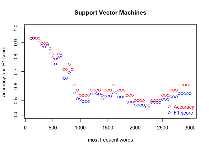
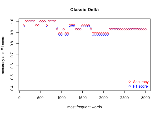
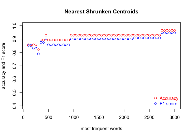
We run the code three times, in order to cover the three classification methods. Each time, we produce a plot. The results are shown in the subsequent figures:


I encourage you to draw the conclusions of the above experiment on your own. One obvious observation is that an optimal number of MFWs might depend on the classification method. Another one is that while some methods show their full potential when fed with a lot of features (MFWs), other methods struggle to pick the signal from noise when the vector of features becomes large.
Conclusion
A solid blog post requires a conclusion. However, I don’t think I can add any conclusive ending here. Rather, I hope this is just the beginning: suffice it to say that a great deal of stylometric experiments are exploiting the above supervised machine-learning scenario in which the final results are reported in the form of accuracy scores and their derivatives, such as recall, precision and the F1 score. Feel encouraged to re-use the concepts discussed in this post, together with the code snippets, in your future experiments. There’s still quite a number of uncharted areas in the field of text analysis!